Difference Between Semi-Log Model and Log-Linear Model (With Examples)
Semi-log Model (also called semi-logarithmic model) involves taking the natural logarithm of only one of the variables (either the dependent or the independent), while the other remains in its original (level) form. This produces a model that is still linear in parameters and can be estimated by ordinary least squares (OLS), but the economic interpretation mixes percentage and absolute changes.
There are two common subtypes:
- Log-lin model (log of dependent variable, linear independent variable):
ln(Y) = β₀ + β₁X + ε- Interpretation: A one-unit increase in X is associated with an approximate 100 × β₁ % change in Y (holding other factors constant).
- Useful when Y grows (or declines) at a constant percentage rate with respect to X (e.g., growth models, wages, prices over time).
- Example: Modeling wages as a function of experience
ln(Wage) = 2.5 + 0.08 × Experience
Each additional year of experience is associated with an ≈ 8% increase in wage.
- Lin-log model (linear dependent variable, log of independent variable):
Y = β₀ + β₁ ln(X) + ε- Interpretation: A 1% increase in X is associated with a β₁ / 100 unit change in Y.
- Useful when the effect of X on Y diminishes as X gets larger (diminishing returns).
- Example: Modeling household food expenditure as a function of income
FoodExp = 500 + 120 × ln(Income)
A 1% increase in income is associated with a 1.20 unit increase in food expenditure.
Log-linear Model (also called double-log, log-log, or constant-elasticity model) takes the natural logarithm of both the dependent and independent variables:
ln(Y) = β₀ + β₁ ln(X) + ε
(or equivalently, Y = e^{β₀} × X^{β₁})
- Interpretation: β₁ is the elasticity — a 1% increase in X is associated with a β₁ % change in Y (constant elasticity).
- Useful when you want to estimate constant proportional responses (e.g., demand functions, production functions).
- Example: Modeling quantity demanded as a function of price
ln(Quantity) = 4.2 – 1.5 × ln(Price)
The price elasticity of demand is –1.5 — a 1% increase in price is associated with a 1.5% decrease in quantity demanded.
Key Distinctions
| Aspect | Semi-log Model | Log-linear Model |
|---|---|---|
| Logs used | Only one variable (Y or X) | Both Y and X |
| Interpretation of β | % change in one variable vs. absolute change in the other | % change in Y vs. % change in X (elasticity) |
| Typical use | Growth rates, diminishing returns | Constant elasticity relationships |
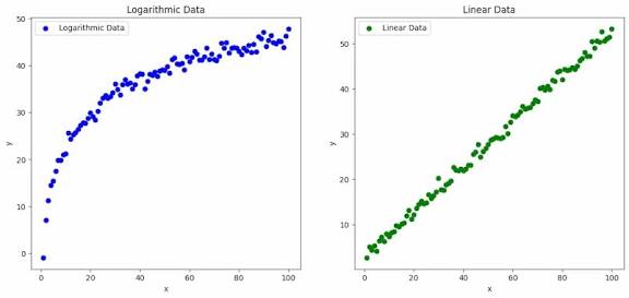
| Plot appearance | Straight line on semi-log paper (one axis logged) | Straight line on log-log paper (both axes logged) |
| Cannot use with | Non-positive values in the logged variable | Non-positive values in either variable |
Both models are linear in parameters, so OLS works directly, but you must be careful when comparing R² or making predictions (e.g., for log-lin or log-linear, you often need to adjust for the retransformation bias when predicting the level of Y).
These functional forms let you capture non-linear relationships in the original variables while keeping the estimation simple and the coefficients economically meaningful.